Performing Scenario Discovery in Python

The purpose of example is to demonstrate how one can do scenario discovery in python. I will demonstrate how we can perform both PRIM in an interactive way, as well as briefly show how to use CART, which is also available in the exploratory modeling workbench. There is ample literature on both CART and PRIM and their relative merits for use in scenario discovery. So I won’t be discussing that here in any detail.

In order to demonstrate the use of the exploratory modeling workbench for scenario discovery, I am using a published example. I am using the data used in the original article by Ben Bryant and Rob Lempert where they first introduced 2010. Ben Bryant kindly made this data available and allowed me to share it. The data comes as a csv file. We can import the data easily using pandas. columns 2 up to and including 10 contain the experimental design, while the classification is presented in column 15

This example is a slightly updated version of a blog post on https://waterprogramming.wordpress.com/2015/08/05/scenario-discovery-in-python/

import pandas as pd

data = pd.read_csv("./data/bryant et al 2010 data.csv", index_col=False)
x = data.iloc[:, 2:11]
y = data.iloc[:, 15].values

The exploratory modeling workbench comes with a separate analysis package. This analysis package contains prim. So let’s import prim. The workbench also has its own logging functionality. We can turn this on to get some more insight into prim while it is running.

from ema_workbench.analysis import prim
from ema_workbench.util import ema_logging

ema_logging.log_to_stderr(ema_logging.INFO);

Next, we need to instantiate the prim algorithm. To mimic the original work of Ben Bryant and Rob Lempert, we set the peeling alpha to 0.1. The peeling alpha determines how much data is peeled off in each iteration of the algorithm. The lower the value, the less data is removed in each iteration. The minimum coverage threshold that a box should meet is set to 0.8. Next, we can use the instantiated algorithm to find a first box.

prim_alg = prim.Prim(x, y, threshold=0.8, peel_alpha=0.1)
box1 = prim_alg.find_box()

[MainProcess/INFO] 882 points remaining, containing 89 cases of interest
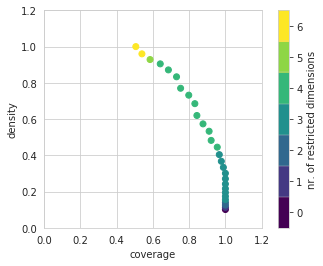
[MainProcess/INFO] mean: 1.0, mass: 0.05102040816326531, coverage: 0.5056179775280899, density: 1.0 restricted_dimensions: 6

Let’s investigate this first box is some detail. A first thing to look at is the trade off between coverage and density. The box has a convenience function for this called show_tradeoff.

box1.show_tradeoff()
plt.show()

Since we are doing this analysis in a notebook, we can take advantage of the interactivity that the browser offers. A relatively recent addition to the python ecosystem is the library altair. Altair can be used to create interactive plots for use in a browser. Altair is an optional dependency for the workbench. If available, we can create the following visual.

box1.inspect_tradeoff()

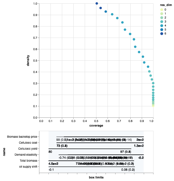
Here we can interactively explore the boxes associated with each point in the density coverage trade-off. It also offers mouse overs for the various points on the trade off curve. Given the id of each point, we can also use the workbench to manually inpect the peeling trajectory. Following Bryant & Lempert, we inspect box 21.

box1.resample(21)

[MainProcess/INFO] resample 0
[MainProcess/INFO] resample 1
[MainProcess/INFO] resample 2
[MainProcess/INFO] resample 3
[MainProcess/INFO] resample 4
[MainProcess/INFO] resample 5
[MainProcess/INFO] resample 6
[MainProcess/INFO] resample 7
[MainProcess/INFO] resample 8
[MainProcess/INFO] resample 9

	reproduce coverage	reproduce density
Total biomass	100.0	100.0
Demand elasticity	100.0	100.0
Biomass backstop price	100.0	100.0
Cellulosic cost	90.0	90.0
Cellulosic yield	20.0	20.0
Electricity coproduction	20.0	20.0
Feedstock distribution	0.0	0.0
Oil elasticity	0.0	0.0
oil supply shift	0.0	0.0

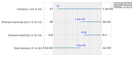
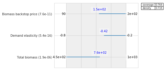
box1.inspect(21)
box1.inspect(21, style="graph")
plt.show()

coverage     0.752809
density      0.770115
id                 21
mass        0.0986395
mean         0.770115
res_dim             4
Name: 21, dtype: object

                            box 21
                               min         max                       qp values
Total biomass           450.000000  755.799988   [-1.0, 4.716968553178765e-06]
Demand elasticity        -0.422000   -0.202000  [1.1849299115762218e-16, -1.0]
Biomass backstop price  150.049995  199.600006   [3.515112530263049e-11, -1.0]
Cellulosic cost          72.650002  133.699997     [0.15741333528927348, -1.0]

If one where to do a detailed comparison with the results reported in the original article, one would see small numerical differences. These differences arise out of subtle differences in implementation. The most important difference is that the exploratory modeling workbench uses a custom objective function inside prim which is different from the one used in the scenario discovery toolkit. Other differences have to do with details about the hill climbing optimization that is used in prim, and in particular how ties are handled in selected the next step. The differences between the two implementations are only numerical, and don’t affect the overarching conclusions drawn from the analysis.

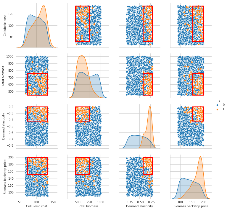
Let’s select this 21 box, and get a more detailed view of what the box looks like. Following Bryant et al., we can use scatter plots for this.

box1.select(21)
fig = box1.show_pairs_scatter(21)
plt.show()

Because the last restriction is not significant, we can choose to drop this restriction from the box.

box1.drop_restriction("Cellulosic cost")
box1.inspect(style="graph")
plt.show()

We have now found a first box that explains over 75% of the cases of interest. Let’s see if we can find a second box that explains the remainder of the cases.

box2 = prim_alg.find_box()

[MainProcess/INFO] 787 points remaining, containing 21 cases of interest
[MainProcess/INFO] box does not meet threshold criteria, value is 0.3541666666666667, returning dump box

As we can see, we are unable to find a second box. The best coverage we can achieve is 0.35, which is well below the specified 0.8 threshold. Let’s look at the final overal results from interactively fitting PRIM to the data. For this, we can use to convenience functions that transform the stats and boxes to pandas data frames.

prim_alg.stats_to_dataframe()

	coverage	density	mass	res_dim
box 1	0.764045	0.715789	0.10771	3
box 2	0.235955	0.026684	0.89229	0

prim_alg.boxes_to_dataframe()

	box 1		box 2
	min	max	min	max
Demand elasticity	-0.422000	-0.202000	-0.8	-0.202000
Biomass backstop price	150.049995	199.600006	90.0	199.600006
Total biomass	450.000000	755.799988	450.0	997.799988

CART

The way of interacting with CART is quite similar to how we setup the prim analysis. We import cart from the analysis package. We instantiate the algorithm, and next fit CART to the data. This is done via the build_tree method.

from ema_workbench.analysis import cart

cart_alg = cart.CART(x, y, 0.05)
cart_alg.build_tree()

/Users/jhkwakkel/miniconda3/lib/python3.6/importlib/_bootstrap.py:219: ImportWarning: can't resolve package from __spec__ or __package__, falling back on __name__ and __path__
  return f(*args, **kwds)
/Users/jhkwakkel/miniconda3/lib/python3.6/importlib/_bootstrap.py:219: ImportWarning: can't resolve package from __spec__ or __package__, falling back on __name__ and __path__
  return f(*args, **kwds)
/Users/jhkwakkel/miniconda3/lib/python3.6/importlib/_bootstrap.py:219: ImportWarning: can't resolve package from __spec__ or __package__, falling back on __name__ and __path__
  return f(*args, **kwds)

Now that we have trained CART on the data, we can investigate its results. Just like PRIM, we can use stats_to_dataframe and boxes_to_dataframe to get an overview.

cart_alg.stats_to_dataframe()

	coverage	density	mass	res dim
box 1	0.011236	0.021739	0.052154	2
box 2	0.000000	0.000000	0.546485	2
box 3	0.000000	0.000000	0.103175	2
box 4	0.044944	0.090909	0.049887	2
box 5	0.224719	0.434783	0.052154	2
box 6	0.112360	0.227273	0.049887	3
box 7	0.000000	0.000000	0.051020	3
box 8	0.606742	0.642857	0.095238	2

cart_alg.boxes_to_dataframe()

	box 1		box 2		box 3		box 4		box 5		box 6		box 7		box 8
	min	max	min	max	min	max	min	max	min	max	min	max	min	max	min	max
Cellulosic yield	80.0	81.649998	81.649998	99.900002	80.000	99.900002	80.000000	99.900002	80.000	99.900002	80.0000	89.049999	89.049999	99.900002	80.000000	99.900002
Demand elasticity	-0.8	-0.439000	-0.800000	-0.439000	-0.439	-0.316500	-0.439000	-0.316500	-0.439	-0.316500	-0.3165	-0.202000	-0.316500	-0.202000	-0.316500	-0.202000
Biomass backstop price	90.0	199.600006	90.000000	199.600006	90.000	144.350006	144.350006	170.750000	170.750	199.600006	90.0000	148.300003	90.000000	148.300003	148.300003	199.600006

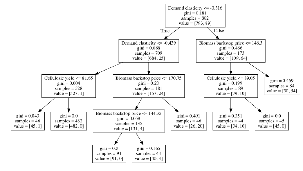
Alternatively, we might want to look at the classification tree directly. For this, we can use the show_tree method.

fig = cart_alg.show_tree()
fig.set_size_inches((18, 12))
plt.show()