Open exploration
In this second tuturial, I will showcase how to use the ema_workbench for performing open exploration. This tuturial will continue with the same example as used in the previous tuturial.
some background
In exploratory modeling, we are interested in understanding how regions in the uncertainty space and/or the decision space map to the whole outcome space, or partitions thereof. There are two general approaches for investigating this mapping. The first one is through systematic sampling of the uncertainty or decision space. This is sometimes also known as open exploration. The second one is to search through the space in a directed manner using some type of optimization approach. This is sometimes also known as directed search.
The workbench support both open exploration and directed search. Both can be applied to investigate the mapping of the uncertainty space and/or the decision space to the outcome space. In most applications, search is used for finding promising mappings from the decision space to the outcome space, while exploration is used to stress test these mappings under a whole range of possible resolutions to the various uncertainties. This need not be the case however. Optimization can be used to discover the worst possible scenario, while sampling can be used to get insight into the sensitivity of outcomes to the various decision levers.
open exploration
To showcase the open exploration functionality, let’s start with a basic example using the Direct Policy Search (DPS) version of the lake problem (Quinn et al 2017). This is the same model as we used in the general introduction. Note that for convenience, I have moved the code for the model to a module called dps_lake_model.py, which I import here for further use.
We are going to simultaneously sample over uncertainties and decision levers. We are going to generate 1000 scenarios and 5 policies, and see how they jointly affect the outcomes. A scenario is understood as a point in the uncertainty space, while a policy is a point in the decision space. The combination of a scenario and a policy is called experiment. The uncertainty space is spanned by uncertainties, while the decision space is spanned by levers.
Both uncertainties and levers are instances of RealParameter (a continuous range), IntegerParameter (a range of integers), or CategoricalParameter (an unorder set of things). By default, the workbench will use Latin Hypercube sampling for generating both the scenarios and the policies. Each policy will be always evaluated over all scenarios (i.e. a full factorial over scenarios and policies).
[1]:
import matplotlib.pyplot as plt
import pandas as pd
import seaborn as sns
from dps_lake_model import lake_model

from ema_workbench import Constant, Model, RealParameter, ScalarOutcome

model = Model("lakeproblem", function=lake_model)

# specify uncertainties
model.uncertainties = [
    RealParameter("b", 0.1, 0.45),
    RealParameter("q", 2.0, 4.5),
    RealParameter("mean", 0.01, 0.05),
    RealParameter("stdev", 0.001, 0.005),
    RealParameter("delta", 0.93, 0.99),
]

# set levers
model.levers = [
    RealParameter("c1", -2, 2),
    RealParameter("c2", -2, 2),
    RealParameter("r1", 0, 2),
    RealParameter("r2", 0, 2),
    RealParameter("w1", 0, 1),
]

# specify outcomes
model.outcomes = [
    ScalarOutcome("max_P"),
    ScalarOutcome("utility"),
    ScalarOutcome("inertia"),
    ScalarOutcome("reliability"),
]

# override some of the defaults of the model
model.constants = [
    Constant("alpha", 0.41),
    Constant("nsamples", 150),
    Constant("myears", 100),
]
[2]:
from ema_workbench import MultiprocessingEvaluator, ema_logging

ema_logging.log_to_stderr(ema_logging.INFO)

# The n_processes=-1 ensures that all cores except 1 are used, which is kept free to keep using the computer
with MultiprocessingEvaluator(model, n_processes=-1) as evaluator:
    # Run 1000 scenarios for 5 policies
    experiments, outcomes = evaluator.perform_experiments(scenarios=1000, policies=5)
[MainProcess/INFO] pool started with 9 workers
[MainProcess/INFO] performing 1000 scenarios * 5 policies * 1 model(s) = 5000 experiments
100%|█████████████████████████████████████| 5000/5000 [00:20<00:00, 238.16it/s]
[MainProcess/INFO] experiments finished
[MainProcess/INFO] terminating pool
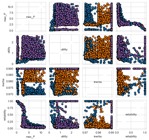
Visual analysis
Having generated these results, the next step is to analyze them and see what we can learn from the results. The workbench comes with a variety of techniques for this analysis. A simple first step is to make a few quick visualizations of the results. The workbench has convenience functions for this, but it also possible to create your own visualizations using the scientific Python stack.
[3]:
from ema_workbench.analysis import pairs_plotting

fig, axes = pairs_plotting.pairs_scatter(
    experiments, outcomes, group_by="policy", legend=False
)
fig.set_size_inches(8, 8)
plt.show()
[MainProcess/INFO] no time dimension found in results
Often, it is convenient to separate the process of performing the experiments from the analysis. To make this possible, the workbench offers convenience functions for storing results to disc and loading them from disc. The workbench will store the results in a tarbal with .csv files and separate metadata files. This is a convenient format that has proven sufficient over the years.
from ema_workbench import save_results
save_results(results, '1000 scenarios 5 policies.tar.gz')

from ema_workbench import load_results
results = load_results('1000 scenarios 5 policies.tar.gz')
advanced analysis
In addition to visual analysis, the workbench comes with a variety of techniques to perform a more in-depth analysis of the results. In addition, other analyses can simply be performed by utilizing the scientific python stack. The workbench comes with
Scenario Discovery, a model driven approach to scenario development
Feature Scoring, a poor man’s alternative to global sensitivity analysis
Dimensional stacking, a quick visual approach drawing on feature scoring to enable scenario discovery. This approach has received limited attention in the literature. The implementation in the workbench replaces the rule mining approach with a feature scoring approach.
Scenario Discovery
A detailed discussion on scenario discovery can be found in an earlier blogpost. For completeness, I provide a code snippet here.
[4]:
from ema_workbench.analysis import prim

x = experiments
y = outcomes["max_P"] < 0.8
prim_alg = prim.Prim(x, y)
box1 = prim_alg.find_box()
[MainProcess/INFO] column model dropped from analysis because it has only one category
[MainProcess/INFO] 5000 points remaining, containing 12497500 cases of interest
[MainProcess/INFO] coverage: 0.6576200417536534, density: 0.984375, mass: 0.064, res_dim: 2,
[5]:
box1.show_tradeoff()
plt.show()
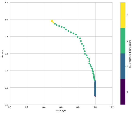
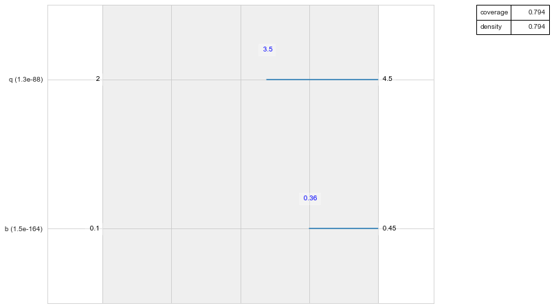
We can inspect any of the points on the trade off curve using the inspect method. As shown, we can show the results either in a table format or in a visual format.
[6]:
box1.inspect(43)
box1.inspect(43, style="graph")
plt.show()
coverage      0.876827
density       0.823529
id           43.000000
k           420.000000
mass          0.102000
mean          0.823529
n           510.000000
res_dim       2.000000
Name: 43, dtype: float64

     box 43
        min       max       qp value qp value
b  0.378259  0.449872  1.910158e-210      NaN
q  3.261761  4.497977   1.764373e-78      NaN
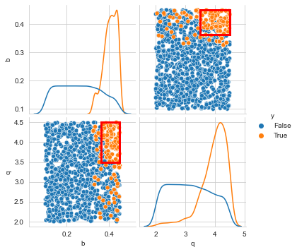
[7]:
box1.show_pairs_scatter(43)
plt.show()
feature scoring
Feature scoring is a family of techniques often used in machine learning to identify the most relevant features to include in a model. This is similar to one of the use cases for global sensitivity analysis, namely factor prioritisation. The main advantage of feature scoring techniques is that they impose no specific constraints on the experimental design, while they can handle real valued, integer valued, and categorical valued parameters. The workbench supports multiple techniques, the most useful of which generally is extra trees (Geurts et al. 2006).
For this example, we run feature scoring for each outcome of interest. We can also run it for a specific outcome if desired. Similarly, we can choose if we want to run in regression mode or classification mode. The later is applicable if the outcome is a categorical variable and the results should be interpreted similar to regional sensitivity analysis results. For more details, see the documentation.
[8]:
from ema_workbench.analysis import feature_scoring

x = experiments
y = outcomes

fs = feature_scoring.get_feature_scores_all(x, y)
sns.heatmap(fs, cmap="viridis", annot=True)
plt.show()
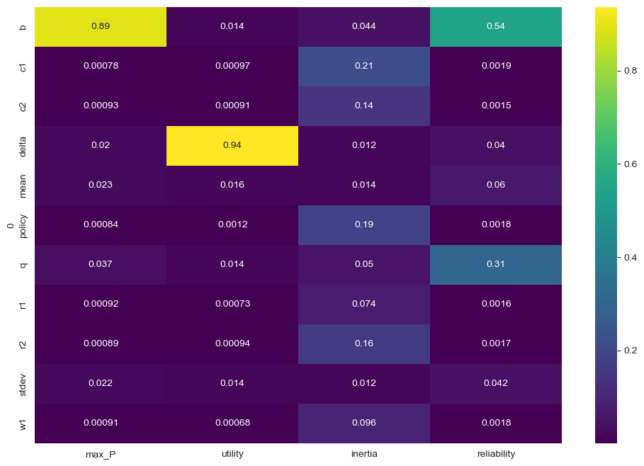
From the results, we see that max_P is primarily influenced by b, while utility is driven by delta, for inertia and reliability the situation is a little bit less clear cut.
The foregoing feature scoring was using the raw values of the outcomes. However, in scenario discovery applications, we are typically dealing with a binary clasification. This might produce slightly different results as demonstrated below
[9]:
from ema_workbench.analysis import RuleInductionType

x = experiments
y = outcomes["max_P"] < 0.8

fs, alg = feature_scoring.get_ex_feature_scores(
    x, y, mode=RuleInductionType.CLASSIFICATION
)
fs.sort_values(ascending=False, by=1)
[9]:
| 1 | |
|---|---|
| 0 | |
| b | 0.497708 |
| q | 0.302515 |
| mean | 0.075032 |
| stdev | 0.056321 |
| delta | 0.054413 |
| c1 | 0.002528 |
| policy | 0.002517 |
| w1 | 0.002407 |
| r2 | 0.002336 |
| c2 | 0.002117 |
| r1 | 0.002109 |
Here we ran extra trees feature scoring on a binary vector for max_P. the b parameter is still important, similar to in the previous case, but the introduction of the binary classifiaction now also highlights some addtional parameters as being potentially relevant.
dimensional stacking
Dimensional stacking was suggested as a more visual approach to scenario discovery. It involves two steps: identifying the most important uncertainties that affect system behavior, and creating a pivot table using the most influential uncertainties. In order to do this, we first need, as in scenario discovery, specify the outcomes that are of interest. The creating of the pivot table involves binning the uncertainties. More details can be found in Suzuki et al. (2015) or by looking through the code in the workbench. Compared to Suzuki et al, the workbench uses feature scoring for determining the most influential uncertainties. The code is set up in a modular way so other approaches to global sensitivity analysis can easily be used as well if so desired.
[10]:
from ema_workbench.analysis import dimensional_stacking

x = experiments
y = outcomes["max_P"] < 0.8
dimensional_stacking.create_pivot_plot(x, y, 2, nbins=3)
plt.show()
[MainProcess/INFO] model dropped from analysis because only a single category
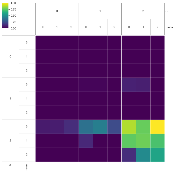
We can see from this visual that if B is high, while Q is high, we have a high concentration of cases where pollution stays below 0.8. The mean and stdev have some limited additional influence. By playing around with an alternative number of bins, or different number of layers, patterns can be coarsened or refined.
regional sensitivity analysis
A fourth approach for supporting scenario discovery is to perform a regional sensitivity analysis. The workbench implements a visual approach based on plotting the empirical CDF given a classification vector. Please look at section 3.4 in Pianosi et al (2016) for more details.
[11]:
from ema_workbench.analysis import regional_sa

sns.set_style("white")

# model is the same across experiments
x = experiments.copy()
y = outcomes["max_P"] < 0.8
fig = regional_sa.plot_cdfs(x, y)
sns.despine()
plt.show()
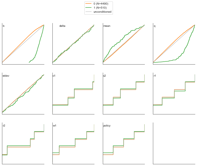
The above results clearly show that both B and Q are important. to a lesser extend, the mean also is relevant.
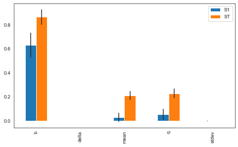
More advanced sampling techniques
The workbench can also be used for more advanced sampling techniques. To achieve this, it relies on SALib. On the workbench side, the only change is to specify the sampler we want to use. Next, we can use SALib directly to perform the analysis. To help with this, the workbench provides a convenience function for generating the problem dict which SALib provides. The example below focusses on performing SOBOL on the uncertainties, but we could do the
exact same thing with the levers instead. The only changes required would be to set lever_sampling instead of uncertainty_sampling, and get the SALib problem dict based on the levers.
[12]:
from SALib.analyze import sobol

from ema_workbench import Samplers
from ema_workbench.em_framework.salib_samplers import get_SALib_problem

with MultiprocessingEvaluator(model) as evaluator:
    sa_results = evaluator.perform_experiments(
        scenarios=1024, uncertainty_sampling=Samplers.SOBOL
    )

experiments, outcomes = sa_results

problem = get_SALib_problem(model.uncertainties)
Si = sobol.analyze(
    problem, outcomes["max_P"], calc_second_order=True, print_to_console=False
)
[MainProcess/INFO] pool started with 10 workers
[MainProcess/INFO] performing 12288 scenarios * 1 policies * 1 model(s) = 12288 experiments
100%|███████████████████████████████████| 12288/12288 [00:45<00:00, 267.62it/s]
[MainProcess/INFO] experiments finished
[MainProcess/INFO] terminating pool
/opt/anaconda3/lib/python3.12/site-packages/SALib/util/__init__.py:274: FutureWarning: unique with argument that is not not a Series, Index, ExtensionArray, or np.ndarray is deprecated and will raise in a future version.
  names = list(pd.unique(groups))
We have now completed the sobol analysis and have calculated the metrics. What remains is to visualize the metrics. Which can be done as shown below, focussing on St and S1. The error bars indicate the confidence intervals.
[13]:
scores_filtered = {k: Si[k] for k in ["ST", "ST_conf", "S1", "S1_conf"]}
Si_df = pd.DataFrame(scores_filtered, index=problem["names"])

sns.set_style("white")
fig, ax = plt.subplots(1)

indices = Si_df[["S1", "ST"]]
err = Si_df[["S1_conf", "ST_conf"]]

indices.plot.bar(yerr=err.values.T, ax=ax)
fig.set_size_inches(8, 6)
fig.subplots_adjust(bottom=0.3)
plt.show()
[ ]: