Tutorials

The code of these examples can be found in the examples package. The first three examples are meant to illustrate the basics of the EMA workbench. How to implement a model, specify its uncertainties and outcomes, and run it. The fourth example is a more extensive illustration based on Pruyt & Hamarat (2010). It shows some more advanced possibilities of the EMA workbench, including one way of handling policies.

• A simple model in Python

• A simple model in Vensim

• A simple model in Excel

• A more elaborate example: Mexican Flu

A simple model in Python

The simplest case is where we have a model available through a python function. For example, imagine we have the simple model.

def some_model(x1=None, x2=None, x3=None):
    return {'y':x1*x2+x3}

In order to control this model from the workbench, we can make use of the Model. We can instantiate a model object, by passing it a name, and the function.

model = Model('simpleModel', function=some_model) #instantiate the model

Next, we need to specify the uncertainties and the outcomes of the model. In this case, the uncertainties are x1, x2, and x3, while the outcome is y. Both uncertainties and outcomes are attributes of the model object, so we can say

#specify uncertainties
model.uncertainties = [RealParameter("x1", 0.1, 10),
                       RealParameter("x2", -0.01,0.01),
                       RealParameter("x3", -0.01,0.01)]
#specify outcomes
model.outcomes = [ScalarOutcome('y')]

Here, we specify that x1 is some value between 0.1, and 10, while both x2 and x3 are somewhere between -0.01 and 0.01. Having implemented this model, we can now investigate the model behavior over the set of uncertainties by simply calling

results = perform_experiments(model, 100)

The function perform_experiments() takes the model we just specified and will execute 100 experiments. By default, these experiments are generated using a Latin Hypercube sampling, but Monte Carlo sampling and Full factorial sampling are also readily available. Read the documentation for perform_experiments() for more details.

The complete code:

"""
Created on 20 dec. 2010

This file illustrated the use the EMA classes for a contrived example
It's main purpose has been to test the parallel processing functionality

.. codeauthor:: jhkwakkel <j.h.kwakkel (at) tudelft (dot) nl>
"""
from ema_workbench import (
    Model,
    RealParameter,
    ScalarOutcome,
    ema_logging,
    perform_experiments,
)


def some_model(x1=None, x2=None, x3=None):
    return {"y": x1 * x2 + x3}


if __name__ == "__main__":
    ema_logging.LOG_FORMAT = "[%(name)s/%(levelname)s/%(processName)s] %(message)s"
    ema_logging.log_to_stderr(ema_logging.INFO)

    model = Model("simpleModel", function=some_model)  # instantiate the model

    # specify uncertainties
    model.uncertainties = [
        RealParameter("x1", 0.1, 10),
        RealParameter("x2", -0.01, 0.01),
        RealParameter("x3", -0.01, 0.01),
    ]
    # specify outcomes
    model.outcomes = [ScalarOutcome("y")]

    results = perform_experiments(model, 100)

A simple model in Vensim

Imagine we have a very simple Vensim model:

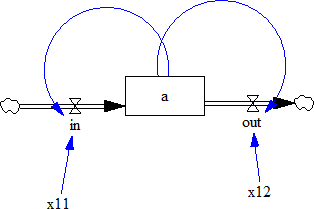
For this example, we assume that ‘x11’ and ‘x12’ are uncertain. The state variable ‘a’ is the outcome of interest. Similar to the previous example, we have to first instantiate a vensim model object, in this case VensimModel. To this end, we need to specify the directory in which the vensim file resides, the name of the vensim file and the name of the model.

wd = r'./models/vensim example'
model = VensimModel("simpleModel", wd=wd, model_file=r'\model.vpm')

Next, we can specify the uncertainties and the outcomes.

model.uncertainties = [RealParameter("x11", 0, 2.5),
                       RealParameter("x12", -2.5, 2.5)]


model.outcomes = [TimeSeriesOutcome('a')]

Note that we are using a TimeSeriesOutcome, because vensim results are time series. We can now simply run this model by calling perform_experiments().

with MultiprocessingEvaluator(model) as evaluator:
results = evaluator.perform_experiments(1000)

We now use a evaluator, which ensures that the code is executed in parallel.

Is it generally good practice to first run a model a small number of times sequentially prior to running in parallel. In this way, bugs etc. can be spotted more easily. To further help with keeping track of what is going on, it is also good practice to make use of the logging functionality provided by the workbench

ema_logging.log_to_stderr(ema_logging.INFO)

Typically, this line appears at the start of the script. When executing the code, messages on progress or on errors will be shown.

The complete code

"""
Created on 3 Jan. 2011

This file illustrated the use the EMA classes for a contrived vensim
example


.. codeauthor:: jhkwakkel <j.h.kwakkel (at) tudelft (dot) nl>
                chamarat <c.hamarat (at) tudelft (dot) nl>
"""
from ema_workbench import (
    TimeSeriesOutcome,
    perform_experiments,
    RealParameter,
    ema_logging,
)

from ema_workbench.connectors.vensim import VensimModel

if __name__ == "__main__":
    # turn on logging
    ema_logging.log_to_stderr(ema_logging.INFO)

    # instantiate a model
    wd = "./models/vensim example"
    vensimModel = VensimModel("simpleModel", wd=wd, model_file="model.vpm")
    vensimModel.uncertainties = [
        RealParameter("x11", 0, 2.5),
        RealParameter("x12", -2.5, 2.5),
    ]

    vensimModel.outcomes = [TimeSeriesOutcome("a")]

    results = perform_experiments(vensimModel, 1000)

A simple model in Excel

In order to perform EMA on an Excel model, one can use the ExcelModel. This base class makes uses of naming cells in Excel to refer to them directly. That is, we can assume that the names of the uncertainties correspond to named cells in Excel, and similarly, that the names of the outcomes correspond to named cells or ranges of cells in Excel. When using this class, make sure that the decimal separator and thousands separator are set correctly in Excel. This can be checked via file > options > advanced. These separators should follow the anglo saxon convention.

"""
Created on 27 Jul. 2011

This file illustrated the use the EMA classes for a model in Excel.

It used the excel file provided by
`A. Sharov <https://home.comcast.net/~sharov/PopEcol/lec10/fullmod.html>`_

This excel file implements a simple predator prey model.

.. codeauthor:: jhkwakkel <j.h.kwakkel (at) tudelft (dot) nl>
"""
from ema_workbench import (
    RealParameter,
    TimeSeriesOutcome,
    ema_logging,
    perform_experiments,
)

from ema_workbench.connectors.excel import ExcelModel
from ema_workbench.em_framework.evaluators import MultiprocessingEvaluator

if __name__ == "__main__":
    ema_logging.log_to_stderr(level=ema_logging.INFO)

    model = ExcelModel(
        "predatorPrey", wd="./models/excelModel", model_file="excel example.xlsx"
    )
    model.uncertainties = [
        RealParameter("K2", 0.01, 0.2),
        # we can refer to a cell in the normal way
        # we can also use named cells
        RealParameter("KKK", 450, 550),
        RealParameter("rP", 0.05, 0.15),
        RealParameter("aaa", 0.00001, 0.25),
        RealParameter("tH", 0.45, 0.55),
        RealParameter("kk", 0.1, 0.3),
    ]

    # specification of the outcomes
    model.outcomes = [
        TimeSeriesOutcome("B4:B1076"),
        # we can refer to a range in the normal way
        TimeSeriesOutcome("P_t"),
    ]  # we can also use named range

    # name of the sheet
    model.default_sheet = "Sheet1"

    with MultiprocessingEvaluator(model) as evaluator:
        results = perform_experiments(
            model, 100, reporting_interval=1, evaluator=evaluator
        )

The example is relatively straight forward. We instantiate an excel model, we specify the uncertainties and the outcomes. We also need to specify the sheet in excel on which the model resides. Next we can call perform_experiments().

Warning

when using named cells. Make sure that the names are defined at the sheet level and not at the workbook level

A more elaborate example: Mexican Flu

This example is derived from Pruyt & Hamarat (2010). This paper presents a small exploratory System Dynamics model related to the dynamics of the 2009 flu pandemic, also known as the Mexican flu, swine flu, or A(H1N1)v. The model was developed in May 2009 in order to quickly foster understanding about the possible dynamics of this new flu variant and to perform rough-cut policy explorations. Later, the model was also used to further develop and illustrate Exploratory Modelling and Analysis.

Mexican Flu: the basic model

In the first days, weeks and months after the first reports about the outbreak of a new flu variant in Mexico and the USA, much remained unknown about the possible dynamics and consequences of the at the time plausible/imminent epidemic/pandemic of the new flu variant, first known as Swine or Mexican flu and known today as Influenza A(H1N1)v.

The exploratory model presented here is small, simple, high-level, data-poor (no complex/special structures nor detailed data beyond crude guestimates), and history-poor.

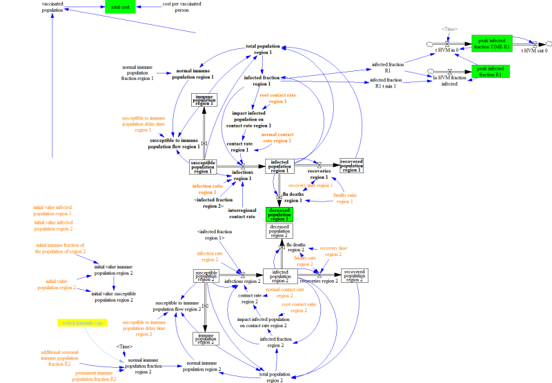
The modelled world is divided in three regions: the Western World, the densely populated Developing World, and the scarcely populated Developing World. Only the two first regions are included in the model because it is assumed that the scarcely populated regions are causally less important for dynamics of flu pandemics. Below, the figure shows the basic stock-and-flow structure. For a more elaborate description of the model, see Pruyt & Hamarat (2010).

Given the various uncertainties about the exact characteristics of the flu, including its fatality rate, the contact rate, the susceptibility of the population, etc. the flu case is an ideal candidate for EMA. One can use EMA to explore the kinds of dynamics that can occur, identify undesirable dynamic, and develop policies targeted at the undesirable dynamics.

In the original paper, Pruyt & Hamarat (2010). recoded the model in Python and performed the analysis in that way. Here we show how the EMA workbench can be connected to Vensim directly.

The flu model was build in Vensim. We can thus use VensimModelS as a base class.

We are interested in two outcomes:

• deceased population region 1: the total number of deaths over the duration of the simulation.

• peak infected fraction: the fraction of the population that is infected.

These are added to self.outcomes, using the TimeSeriesOutcome class.

The table below is adapted from Pruyt & Hamarat (2010). It shows the uncertainties, and their bounds. These are added to self.uncertainties as ParameterUncertainty instances.

Parameter	Lower Limit	Upper Limit
additional seasonal immune population fraction region 1	0.0	0.5
additional seasonal immune population fraction region 2	0.0	0.5
fatality ratio region 1	0.0001	0.1
fatality ratio region 2	0.0001	0.1
initial immune fraction of the population of region 1	0.0	0.5
initial immune fraction of the population of region 2	0.0	0.5
normal interregional contact rate	0.0	0.9
permanent immune population fraction region 1	0.0	0.5
permanent immune population fraction region 2	0.0	0.5
recovery time region 1	0.2	0.8
recovery time region 2	0.2	0.8
root contact rate region 1	1.0	10.0
root contact rate region 2	1.0	10.0
infection ratio region 1	0.0	0.1
infection ratio region 2	0.0	0.1
normal contact rate region 1	10	200
normal contact rate region 2	10	200

Together, this results in the following code:

"""
Created on 20 May, 2011

This module shows how you can use vensim models directly
instead of coding the model in Python. The underlying case
is the same as used in fluExample

.. codeauthor:: jhkwakkel <j.h.kwakkel (at) tudelft (dot) nl>
                epruyt <e.pruyt (at) tudelft (dot) nl>
"""
from ema_workbench import (
    RealParameter,
    TimeSeriesOutcome,
    ema_logging,
    perform_experiments,
    MultiprocessingEvaluator,
)

from ema_workbench.connectors.vensim import VensimModel

if __name__ == "__main__":
    ema_logging.log_to_stderr(ema_logging.INFO)

    model = VensimModel(
        "fluCase", wd="./models/flu", model_file="FLUvensimV1basecase.vpm"
    )

    # outcomes
    model.outcomes = [
        TimeSeriesOutcome("deceased population region 1"),
        TimeSeriesOutcome("infected fraction R1"),
    ]

    # Plain Parametric Uncertainties
    model.uncertainties = [
        RealParameter("additional seasonal immune population fraction R1", 0, 0.5),
        RealParameter("additional seasonal immune population fraction R2", 0, 0.5),
        RealParameter("fatality ratio region 1", 0.0001, 0.1),
        RealParameter("fatality rate region 2", 0.0001, 0.1),
        RealParameter("initial immune fraction of the population of region 1", 0, 0.5),
        RealParameter("initial immune fraction of the population of region 2", 0, 0.5),
        RealParameter("normal interregional contact rate", 0, 0.9),
        RealParameter("permanent immune population fraction R1", 0, 0.5),
        RealParameter("permanent immune population fraction R2", 0, 0.5),
        RealParameter("recovery time region 1", 0.1, 0.75),
        RealParameter("recovery time region 2", 0.1, 0.75),
        RealParameter("susceptible to immune population delay time region 1", 0.5, 2),
        RealParameter("susceptible to immune population delay time region 2", 0.5, 2),
        RealParameter("root contact rate region 1", 0.01, 5),
        RealParameter("root contact ratio region 2", 0.01, 5),
        RealParameter("infection ratio region 1", 0, 0.15),
        RealParameter("infection rate region 2", 0, 0.15),
        RealParameter("normal contact rate region 1", 10, 100),
        RealParameter("normal contact rate region 2", 10, 200),
    ]

    nr_experiments = 10
    with MultiprocessingEvaluator(model) as evaluator:
        results = perform_experiments(model, nr_experiments, evaluator=evaluator)

We have now instantiated the model, specified the uncertain factors and outcomes and run the model. We now have generated a dataset of results and can proceed to analyse the results using various analysis scripts. As a first step, one can look at the individual runs using a line plot using lines(). See plotting for some more visualizations using results from performing EMA on FluModel.

import matplotlib.pyplot as plt
from ema_workbench.analysis.plotting import lines

figure = lines(results, density=True) #show lines, and end state density
plt.show() #show figure

generates the following figure:

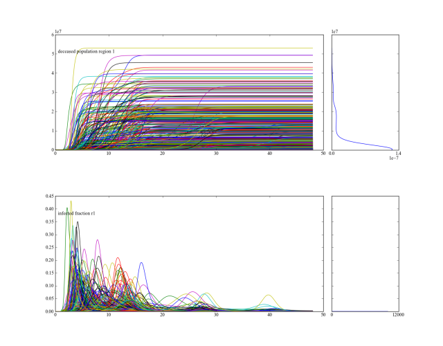
From this figure, one can deduce that across the ensemble of possible futures, there is a subset of runs with a substantial amount of deaths. We can zoom in on those cases, identify their conditions for occurring, and use this insight for policy design.

For further analysis, it is generally convenient, to generate the results for a series of experiments and save these results. One can then use these saved results in various analysis scripts.

from ema_workbench import save_results
save_results(results, r'./1000 runs.tar.gz')

The above code snippet shows how we can use save_results() for saving the results of our experiments. save_results() stores the as csv files in a tarbal.

Mexican Flu: policies

For this paper, policies were developed by using the system understanding of the analysts.

static policy

adaptive policy

running the policies

In order to be able to run the models with the policies and to compare their results with the no policy case, we need to specify the policies

#add policies
policies = [Policy('no policy',
                   model_file=r'/FLUvensimV1basecase.vpm'),
            Policy('static policy',
                   model_file=r'/FLUvensimV1static.vpm'),
            Policy('adaptive policy',
                   model_file=r'/FLUvensimV1dynamic.vpm')
            ]

In this case, we have chosen to have the policies implemented in separate vensim files. Policies require a name, and can take any other keyword arguments you like. If the keyword matches an attribute on the model object, it will be updated, so model_file is an attribute on the vensim model. When executing the policies, we update this attribute for each policy. We can pass these policies to perform_experiment() as an additional keyword argument

results = perform_experiments(model, 1000, policies=policies)

We can now proceed in the same way as before, and perform a series of experiments. Together, this results in the following code:

"""
Created on 20 May, 2011

This module shows how you can use vensim models directly
instead of coding the model in Python. The underlying case
is the same as used in fluExample

.. codeauthor:: jhkwakkel <j.h.kwakkel (at) tudelft (dot) nl>
                epruyt <e.pruyt (at) tudelft (dot) nl>
"""
import numpy as np

from ema_workbench import (
    RealParameter,
    TimeSeriesOutcome,
    ema_logging,
    ScalarOutcome,
    perform_experiments,
)
from ema_workbench.connectors.vensim import VensimModel
from ema_workbench.em_framework.parameters import Policy

if __name__ == "__main__":
    ema_logging.log_to_stderr(ema_logging.INFO)

    model = VensimModel(
        "fluCase", wd=r"./models/flu", model_file=r"FLUvensimV1basecase.vpm"
    )

    # outcomes
    model.outcomes = [
        TimeSeriesOutcome("deceased population region 1"),
        TimeSeriesOutcome("infected fraction R1"),
        ScalarOutcome(
            "max infection fraction",
            variable_name="infected fraction R1",
            function=np.max,
        ),
    ]

    # Plain Parametric Uncertainties
    model.uncertainties = [
        RealParameter("additional seasonal immune population fraction R1", 0, 0.5),
        RealParameter("additional seasonal immune population fraction R2", 0, 0.5),
        RealParameter("fatality ratio region 1", 0.0001, 0.1),
        RealParameter("fatality rate region 2", 0.0001, 0.1),
        RealParameter("initial immune fraction of the population of region 1", 0, 0.5),
        RealParameter("initial immune fraction of the population of region 2", 0, 0.5),
        RealParameter("normal interregional contact rate", 0, 0.9),
        RealParameter("permanent immune population fraction R1", 0, 0.5),
        RealParameter("permanent immune population fraction R2", 0, 0.5),
        RealParameter("recovery time region 1", 0.1, 0.75),
        RealParameter("recovery time region 2", 0.1, 0.75),
        RealParameter("susceptible to immune population delay time region 1", 0.5, 2),
        RealParameter("susceptible to immune population delay time region 2", 0.5, 2),
        RealParameter("root contact rate region 1", 0.01, 5),
        RealParameter("root contact ratio region 2", 0.01, 5),
        RealParameter("infection ratio region 1", 0, 0.15),
        RealParameter("infection rate region 2", 0, 0.15),
        RealParameter("normal contact rate region 1", 10, 100),
        RealParameter("normal contact rate region 2", 10, 200),
    ]

    # add policies
    policies = [
        Policy("no policy", model_file=r"FLUvensimV1basecase.vpm"),
        Policy("static policy", model_file=r"FLUvensimV1static.vpm"),
        Policy("adaptive policy", model_file=r"FLUvensimV1dynamic.vpm"),
    ]

    results = perform_experiments(model, 1000, policies=policies)

comparison of results

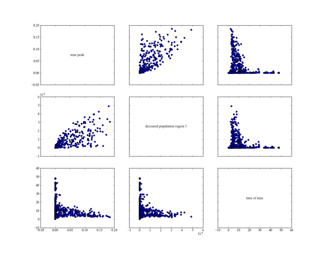
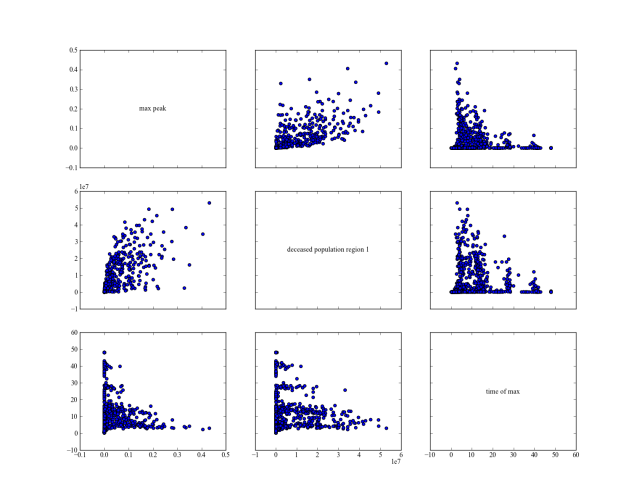
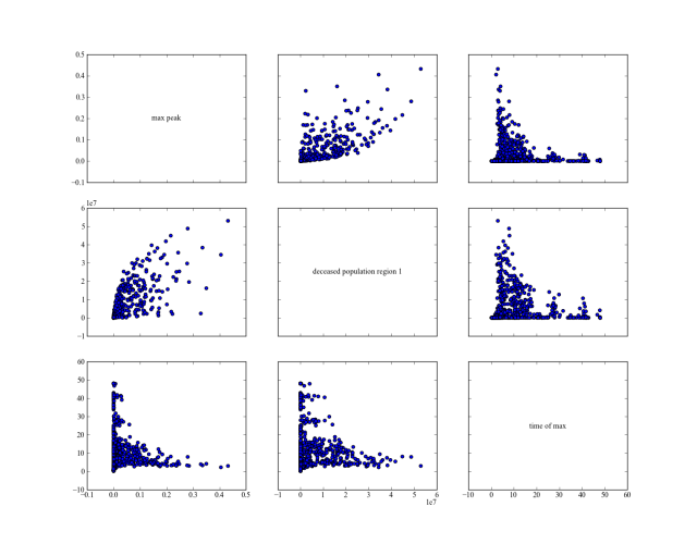
Using the following script, we reproduce figures similar to the 3D figures in Pruyt & Hamarat (2010). But using pairs_scatter(). It shows for the three different policies their behavior on the total number of deaths, the height of the heigest peak of the pandemic, and the point in time at which this peak was reached.

"""
Created on 20 sep. 2011

.. codeauthor:: jhkwakkel <j.h.kwakkel (at) tudelft (dot) nl>
"""
import matplotlib.pyplot as plt
import numpy as np

from ema_workbench import load_results, ema_logging
from ema_workbench.analysis.pairs_plotting import (
    pairs_lines,
    pairs_scatter,
    pairs_density,
)

ema_logging.log_to_stderr(level=ema_logging.DEFAULT_LEVEL)

# load the data
fh = "./data/1000 flu cases no policy.tar.gz"
experiments, outcomes = load_results(fh)

# transform the results to the required format
# that is, we want to know the max peak and the casualties at the end of the
# run
tr = {}

# get time and remove it from the dict
time = outcomes.pop("TIME")

for key, value in outcomes.items():
    if key == "deceased population region 1":
        tr[key] = value[:, -1]  # we want the end value
    else:
        # we want the maximum value of the peak
        max_peak = np.max(value, axis=1)
        tr["max peak"] = max_peak

        # we want the time at which the maximum occurred
        # the code here is a bit obscure, I don't know why the transpose
        # of value is needed. This however does produce the appropriate results
        logical = value.T == np.max(value, axis=1)
        tr["time of max"] = time[logical.T]

pairs_scatter(experiments, tr, filter_scalar=False)
pairs_lines(experiments, outcomes)
pairs_density(experiments, tr, filter_scalar=False)
plt.show()

no policy

static policy

adaptive policy